Last week, I virtually dropped by University of Wisconsin-Madison for a webinar on tidymodels. Heading into the holidays, I thought a fun example problem might be to try and predict flight delays using flights data from Madison’s airport. This is a very, very difficult modeling problem, and the results aren’t very impressive, but it’s a fun one nonetheless.
I’ve collected some data on all of the outbound flights from Madison, Wisconsin in 2022. In this blog post, we’ll use predictors based on the weather, plane, airline, and flight duration to try to predict whether a flight will be delayed or not. To do so, we will split up the source data and then train models in two stages:
Round 1) Try out a variety of models, from a logistic regression to a boosted tree to a neural network, using a grid search for each.
Round 2) Try out more advanced search techniques for the model that seems the most performant in Round 1).
Once we’ve trained the final model fit, we can assess the predictive performance on the test set and prepare the model to be deployed.
Setup
First, loading the tidyverse and tidymodels, along with a few additional tidymodels extension packages:
The finetune package will give us additional tuning functionality, while the bonsai and baguette packages provide support for additional model types.
tidymodels supports a number of R frameworks for parallel computing:
# loading needed packages:
library(doMC)
library(parallelly)

# check out how many cores we have:
availableCores()
system
10 # register those cores so that tidymodels can see them:
registerDoMC(cores = max(1, availableCores() - 1))With a multi-core setup registered, tidymodels will now make use of all of the cores on my computer for expensive computations.
Data Import
We’ll make use of a dataset, msnflights22, containing data on all outbound flights from Madison, Wisconsin in 2022.
load("data/msnflights22.rda")

msnflights22
# A tibble: 10,754 × 14
delayed airline flight origin destination date hour plane distance
<fct> <chr> <fct> <fct> <fct> <date> <dbl> <fct> <dbl>
1 No Endeavor A… 51 MSN ATL 2022-01-01 5 N901… 707
2 No PSA Airlin… 59 MSN CLT 2022-01-01 6 N570… 708
3 No Envoy Air 27 MSN MIA 2022-01-01 6 N280… 1300
4 No American A… 3 MSN PHX 2022-01-01 6 N662… 1396
5 Yes American A… 16 MSN DFW 2022-01-01 7 N826… 821
6 No SkyWest Ai… 26 MSN MSP 2022-01-01 7 N282… 228
7 No United Air… 1 MSN EWR 2022-01-01 7 <NA> 799
8 No United Air… 6 MSN DEN 2022-01-01 8 N830… 826
9 No Republic A… 29 MSN ORD 2022-01-01 8 N654… 109
10 No Endeavor A… 62 MSN DTW 2022-01-01 9 N582… 311
# ℹ 10,744 more rows
# ℹ 5 more variables: duration <dbl>, wind_speed <dbl>, precip <dbl>,
# visibility <dbl>, plane_year <int>You can make your own flights data using the anyflights package! The query_data.R file contains the code used to generate this dataset.
We’d like to model delayed, a binary outcome variable giving whether a given flight was delayed by 10 or more minutes.
# summarize counts of the outcome variable
ggplot(msnflights22) +
  aes(x = delayed) +
  geom_bar(fill = "#4A7862")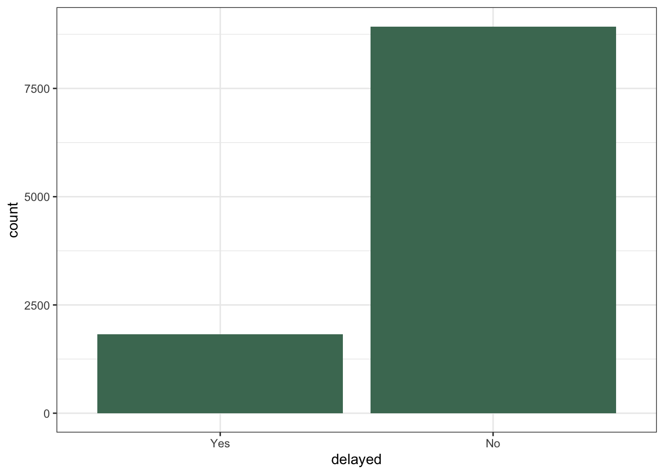
Predicting flight delays seems quite difficult given the data we have access to. For example, plotting whether a flight is delayed based on precipitation and wind speed:
# plot 2 predictors, colored by the outcome
msnflights22 %>%
  filter(precip != 0) %>%
  ggplot() +
  aes(x = wind_speed, y = precip, color = delayed) +
  geom_jitter()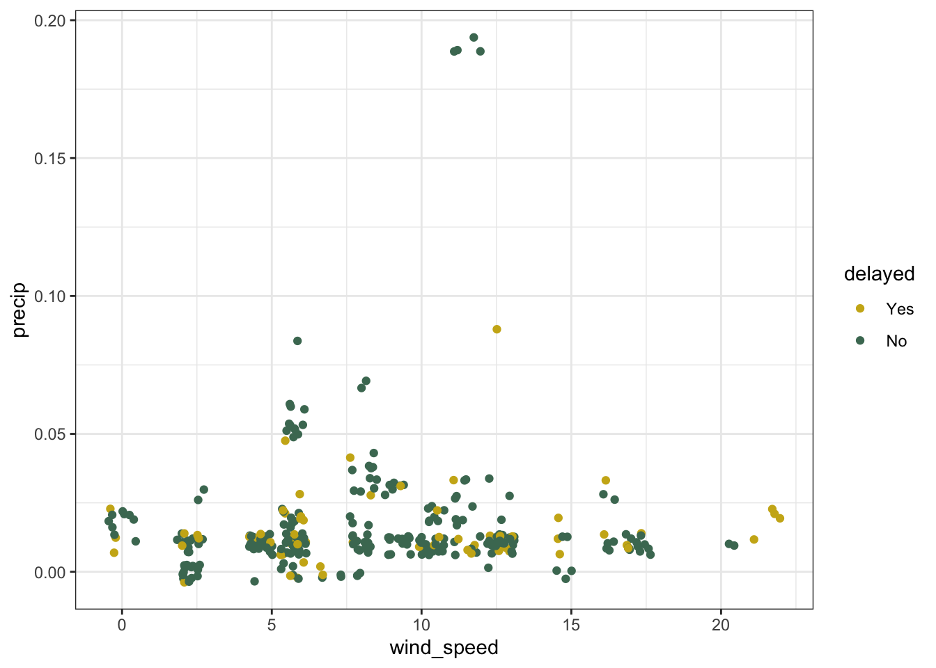
Looks like there’s a bit of signal in the time of the day of the flight, but those higher-proportion-delayed hours also have quite a bit fewer flights (and thus more variation):
(
  ggplot(msnflights22, aes(x = hour, fill = delayed)) +
  geom_bar()
) /
(
  ggplot(msnflights22, aes(x = hour, fill = delayed)) +
  geom_bar(position = "fill") + labs(y = "proportion")
)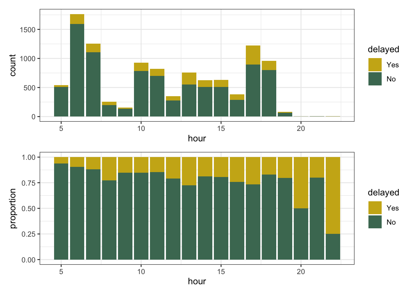
A machine learning model may be able to get some traction here, though.
Splitting up data
We split data into training and testing sets so that, once we’ve trained our final model, we can get an honest assessment of the model’s performance. Since this data is a time series, we’ll allot the first ~10 months to training and the remainder to testing:
# set the seed for random number generation
set.seed(1)

# split the flights data into...
flights_split <- initial_time_split(msnflights22, prop = 5/6)
# training [jan - oct]
flights_train <- training(flights_split)
# ...and testing  [nov - dec]
flights_test <- testing(flights_split)
Then, we’ll resample the training data using a sliding period.
A sliding period is a cross-fold validation technique that takes times into account. The tidymodels packages support more basic resampling schemes like bootstrapping and v-fold cross-validation as well—see the rsample package’s website.
We create 8 folds, where in each fold the analysis set is a 2-month sample of data and the assessment set is the single month following.
set.seed(1)
flights_folds <-
  sliding_period(
    flights_train,
    index = date,
    "month",
    lookback = 1,
    assess_stop = 1
  )

flights_folds
# Sliding period resampling
# A tibble: 8 × 2
splits id
<list> <chr>
1 <split [1783/988]> Slice1
2 <split [1833/819]> Slice2
3 <split [1807/930]> Slice3
4 <split [1749/901]> Slice4
5 <split [1831/906]> Slice5
6 <split [1807/920]> Slice6
7 <split [1826/888]> Slice7
8 <split [1808/826]> Slice8For example, in the second split,
# training: february, march, april
training(flights_folds$splits[[2]]) %>% pull(date) %>% month() %>% unique()
[1] 2 3[1] 4What months will be in the training and testing sets in the third fold?
Defining our modeling strategies
Our basic strategy is to first try out a bunch of different modeling approaches, and once we have an initial sense for how they perform, delve further into the one that looks the most promising.
We first define a few recipes, which specify how to process the inputted data in such a way that machine learning models will know how to work with predictors:
recipe_basic <-
  recipe(delayed ~ ., flights_train) %>%
  step_nzv(all_predictors())

recipe_normalize <-
  recipe_basic %>%
  step_YeoJohnson(all_double_predictors()) %>%
  step_normalize(all_double_predictors())

recipe_pca <-
  recipe_normalize %>%
  step_impute_median(all_numeric_predictors()) %>%
  step_impute_mode(all_nominal_predictors()) %>%
  step_pca(all_numeric_predictors(), num_comp = tune())
These recipes vary in complexity, from basic checks on the input data to advanced feature engineering techniques like principal component analysis.
These preprocessors make use of predictors based on weather. Given that prediction models are only well-defined when trained using variables that are available at prediction time, in what use cases would this model be useful?
We also define several model specifications. tidymodels comes with support for all sorts of machine learning algorithms, from neural networks to LightGBM boosted trees to plain old logistic regression:
spec_lr <-
  logistic_reg() %>%
  set_mode("classification")

spec_bm <-
  bag_mars(num_terms = tune(), prod_degree = tune()) %>%
  set_engine("earth") %>%
  set_mode("classification")

spec_bt <-
  bag_tree(cost_complexity = tune(), tree_depth = tune(), min_n = tune()) %>%
  set_engine("rpart") %>%
  set_mode("classification")

spec_nn <-
  mlp(hidden_units = tune(), penalty = tune(), epochs = tune()) %>%
  set_engine("nnet", MaxNWts = 15000) %>%
  set_mode("classification")

spec_svm <-
  svm_rbf(cost = tune(), rbf_sigma = tune(), margin = tune()) %>%
  set_mode("classification")

spec_lgb <-
  boost_tree(trees = tune(), min_n = tune(), tree_depth = tune(),
             learn_rate = tune(), stop_iter = 10) %>%
  set_engine("lightgbm") %>%
  set_mode("classification")
Note how similar the code for each of these model specifications looks! tidymodels takes care of the “translation” from our unified syntax to the code that these algorithms expect.
If typing all of these out seems cumbersome to you, or you’re not sure how to define a model specification that makes sense for your data, the usemodels RStudio addin may help!
Evaluating models: round 1
We’ll pair machine learning models with the recipes that make the most sense for them using workflow sets:
wf_set <-
  # pair the basic recipe with a boosted tree and logistic regression
  workflow_set(
    preproc = list(basic = recipe_basic),
    models = list(boost_tree = spec_lgb, logistic_reg = spec_lr)
  ) %>%
  # pair the recipe that centers and scales input variables
  # with the bagged models, support vector machine, and neural network
  bind_rows(
    workflow_set(
      preproc = list(normalize = recipe_normalize),
      models = list(
        bag_tree = spec_bt,
        bag_mars = spec_bm,
        svm_rbf = spec_svm,
        mlp = spec_nn
      )
    )
  ) %>%
  # pair those same models with a more involved, principal component
  # analysis preprocessor
  bind_rows(
    workflow_set(
      preproc = list(pca = recipe_pca),
      models = list(
        bag_tree = spec_bt,
        bag_mars = spec_bm,
        svm_rbf = spec_svm,
        mlp = spec_nn
      )
    )
  )

wf_set
# A workflow set/tibble: 10 × 4
wflow_id info option result
<chr> <list> <list> <list>
1 basic_boost_tree <tibble [1 × 4]> <opts[0]> <list [0]>
2 basic_logistic_reg <tibble [1 × 4]> <opts[0]> <list [0]>
3 normalize_bag_tree <tibble [1 × 4]> <opts[0]> <list [0]>
4 normalize_bag_mars <tibble [1 × 4]> <opts[0]> <list [0]>
5 normalize_svm_rbf <tibble [1 × 4]> <opts[0]> <list [0]>
6 normalize_mlp <tibble [1 × 4]> <opts[0]> <list [0]>
7 pca_bag_tree <tibble [1 × 4]> <opts[0]> <list [0]>
8 pca_bag_mars <tibble [1 × 4]> <opts[0]> <list [0]>
9 pca_svm_rbf <tibble [1 × 4]> <opts[0]> <list [0]>
10 pca_mlp <tibble [1 × 4]> <opts[0]> <list [0]>Now that we’ve defined each of our modeling configurations, we’ll fit them to the resamples we defined earlier. Here, tune_grid() is applied to each workflow in the workflow set, testing out a set of tuning parameter values for each workflow and assessing the resulting fit.
wf_set_fit <-
  workflow_map(
    wf_set,
    fn = "tune_grid",
    verbose = TRUE,
    seed = 1,
    resamples = flights_folds,
    control = control_grid(parallel_over = "everything")
)workflow_map() is calling tune_grid() on each modeling workflow we’ve created. You can read more about tune_grid() here.
wf_set_fit# A workflow set/tibble: 8 × 4
wflow_id info option result
<chr> <list> <list> <list>
1 basic_boost_tree <tibble [1 × 4]> <opts[2]> <tune[+]>
2 normalize_bag_tree <tibble [1 × 4]> <opts[2]> <tune[+]>
3 normalize_bag_mars <tibble [1 × 4]> <opts[2]> <tune[+]>
4 normalize_mlp <tibble [1 × 4]> <opts[2]> <tune[+]>
5 pca_bag_tree <tibble [1 × 4]> <opts[2]> <tune[+]>
6 pca_bag_mars <tibble [1 × 4]> <opts[2]> <tune[+]>
7 pca_svm_rbf <tibble [1 × 4]> <opts[2]> <tune[+]>
8 pca_mlp <tibble [1 × 4]> <opts[2]> <tune[+]>Note that the result column that was previously empty in wf_set now contains various tuning results, denoted by <tune[+]>, in wf_set_fit.
There’s a few rows missing here; I filtered out results that failed to tune.
Collecting the information on performance from the resulting object:
# first look at metrics:
metrics_wf_set <- collect_metrics(wf_set_fit)
# extract the top roc_auc values
metrics_wf_set %>%
filter(.metric == "roc_auc") %>%
arrange(desc(mean)) %>%
select(wflow_id, mean, n)# A tibble: 71 × 3
wflow_id mean n
<chr> <dbl> <int>
1 normalize_bag_mars 0.615 8
2 normalize_bag_mars 0.613 8
3 pca_svm_rbf 0.608 8
4 normalize_bag_mars 0.606 8
5 pca_bag_mars 0.604 8
6 normalize_bag_mars 0.603 8
7 pca_svm_rbf 0.603 8
8 pca_bag_mars 0.601 8
9 pca_bag_mars 0.598 8
10 normalize_bag_mars 0.598 8
# ℹ 61 more rowsAlternatively, we can use the autoplot() method for workflow sets to visualize the same results:
autoplot(wf_set_fit)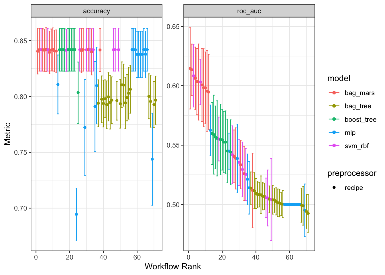
In terms of accuracy(), several of the models we evaluated performed quite well (with values near the event rate). With respect to roc_auc(), though, we can see that the bagged MARS models were clear winners.
Evaluating models: round 2
It looks like a bagged MARS model with centered and scaled predictors was considerably more performant than the other proposed models. Let’s work with those MARS results and see if we can make any further improvements to performance:
mars_res <- extract_workflow_set_result(wf_set_fit, "normalize_bag_mars")

mars_wflow <-
  workflow() %>%
  add_recipe(recipe_normalize) %>%
  add_model(spec_bm)

mars_sim_anneal_fit <-
  tune_sim_anneal(
    object = mars_wflow,
    resamples = flights_folds,
    iter = 10,
    initial = mars_res,
    control = control_sim_anneal(verbose = TRUE, parallel_over = "everything")
  )
Looks like we did make a small improvement, though the model still doesn’t do much better than randomly guessing:
# A tibble: 10 × 8
   num_terms prod_degree .metric .estimator .config  mean     n std_err
       <int>       <int> <chr>   <chr>      <chr>   <dbl> <int>   <dbl>
 1         4           2 roc_auc binary     Iter1   0.619     8  0.0191
 2         3           2 roc_auc binary     Iter6   0.612     8  0.0249
 3         5           2 roc_auc binary     Iter8   0.610     8  0.0185
 4         4           1 roc_auc binary     Iter9   0.606     8  0.0154
 5         3           2 roc_auc binary     Iter4   0.605     8  0.0211
 6         4           1 roc_auc binary     Iter7   0.595     8  0.0205
 7         3           2 roc_auc binary     Iter10  0.594     8  0.0192
 8         3           1 roc_auc binary     Iter2   0.591     8  0.0248
 9         2           1 roc_auc binary     Iter5   0.559     8  0.0183
10         2           2 roc_auc binary     Iter3   0.555     8  0.0175
Just like the workflow set result from before, the simulated annealing result also has an autoplot() method:
autoplot(mars_sim_anneal_fit)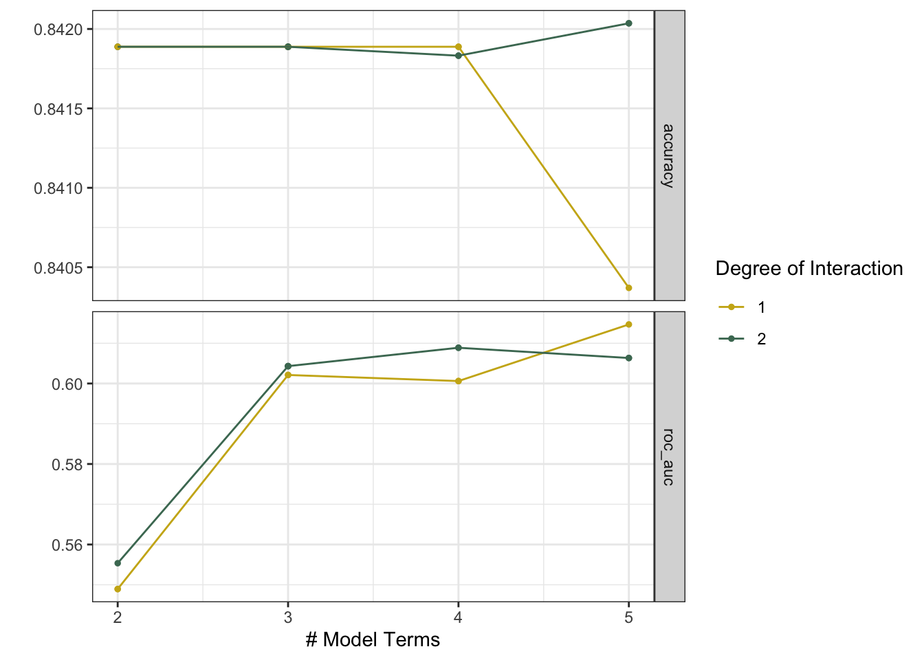
We can now train the model with the most optimal performance in cross-validation on the entire training set.
The final model fit
The last_fit() function will take care of fitting the most performant model specification to the whole training dataset and evaluating it’s performance with the test set:
mars_final_fit <-
  mars_sim_anneal_fit %>%
  # extract the best hyperparameter configuration
  select_best("roc_auc") %>%
  # attach it to the general workflow
  finalize_workflow(mars_wflow, .) %>%
  # evaluate the final workflow on the train/test split
  last_fit(flights_split)

mars_final_fit
The test set roc_auc() for this model was 0.625. The final fitted workflow can be extracted from mars_final_fit and is ready to predict on new data:
final_fit <- extract_workflow(mars_final_fit)Deploying to Connect
From here, all we’d need to do to deploy our fitted model is pass it off to vetiver for deployment to Posit Connect:
final_fit_vetiver <- vetiver_model(final_fit, "simon.couch/flights")

board <- board_connect()

vetiver_pin_write(board, final_fit_vetiver)

vetiver_deploy_rsconnect(board, "simon.couch/flights")