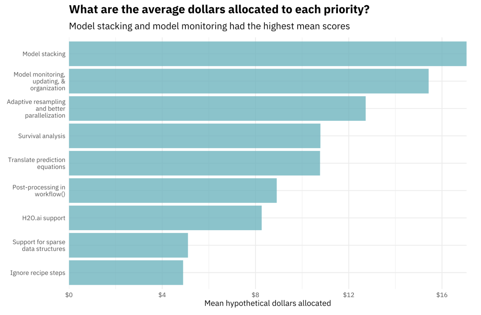
A few months ago, the tidymodels team coordinated a community survey to get a sense for what users most wanted to see next in the tidymodels ecosystem. One resounding theme from responses was that tidymodels users wanted a framework for tidymodels-aligned model stacking.
I spent the latter half of my Summer 2020 internship with RStudio working on a package for model stacking in the tidymodels, and have since continued this work as the subject of my undergraduate thesis at Reed College.
Model stacking is an ensembling technique that involves training a model to combine the outputs of many diverse statistical models. The stacks package implements a grammar for tidymodels-aligned model stacking.
To demonstrate how to build an ensemble with stacks, we’ll make use of this week’s TidyTuesday data on Canadian wind turbines. From a recent article from the National Observer by Carl Meyer:
Natural Resources Canada has published the Canadian Wind Turbine Database, which contains the precise latitude and longitude of every turbine, along with details like its dimensions, its power output, its manufacturer and the date it was commissioned. There is also an interactive map… “For the first time, Canadians have access to centralized geographic and technical information on individual wind turbines that make up individual wind farms, (which) were all collected prior to now very much on an aggregated basis,” said Tom Levy, senior wind engineer at the federal Natural Resources Department.
Making use of the stacks package, we’ll build a stacked ensemble model to predict turbine capacity in kilowatts based on turbine characteristics.
We’ll load up needed packages and then get going!
library(tidyverse)
library(tidymodels)
In addition to the tidyverse and tidymodels, we’ll load the stacks package. If you haven’t installed the stacks package before, you can use the following code:
remotes::install_github("tidymodels/stacks", ref = "main")You might be prompted to update some packages from the tidymodels; make sure to update to the developmental version of tune. Now, loading the stacks package:
library(stacks)Data
wind_raw <- read_csv('https://raw.githubusercontent.com/rfordatascience/tidytuesday/master/data/2020/2020-10-27/wind-turbine.csv')First thing, we’ll subset down to variables that we’ll use in the stacked ensemble model. For the most part, I’m just getting rid of ID variables and qualitative variables with a lot of levels.
wind <-
  wind_raw %>%
  select(
    province_territory,
    total_project_capacity_mw,
    turbine_rated_capacity_kw = turbine_rated_capacity_k_w,
    rotor_diameter_m,
    hub_height_m,
    year = commissioning_date
  ) %>%
  group_by(province_territory) %>%
  mutate(
    year = as.numeric(year),
    province_territory = case_when(
      n() < 50 ~ "Other",
      TRUE ~ province_territory
    )
  ) %>%
  filter(!is.na(year)) %>%
  ungroup()
Creating Model Definitions
At the highest level, ensembles are formed from model definitions. In this package, model definitions are an instance of a minimal workflow, containing a model specification (as defined in the parsnip package) and, optionally, a preprocessor (as defined in the recipes package). Model definitions specify the form of candidate ensemble members.

Note that the diagrams will refer to a K-nearest neighbors, linear regression, and neural network. In these examples, we’ll use different model types!
Defining the constituent model definitions is undoubtedly the longest part of building an ensemble with stacks. If you’re familiar with tidymodels “proper,” you’re probably fine to skip this section, with one note: you’ll need to save the assessment set predictions and workflow utilized in your tune_grid(), tune_bayes(), or fit_resamples() objects by setting the control arguments save_pred = TRUE and save_workflow = TRUE. Note the use of the control_stack_*() convenience functions below!
To be used in the same ensemble, each of these model definitions must share the same resample. This rsample rset object, when paired with the model definitions, can be used to generate the tuning/fitting results objects for the candidate ensemble members with tune.

We’ll first start out with splitting up the training data, generating resamples, and setting some options that will be used by each model definition.
Splitting up the wind data using rsample:
# split into training and testing sets
set.seed(1)
wind_split <- initial_split(wind)
wind_train <- training(wind_split)
wind_test  <- testing(wind_split)

# use a 5-fold cross-validation
set.seed(1)
folds <- rsample::vfold_cv(wind_train, v = 5)
Now, with the recipes and workflows packages, we’ll set up a foundation for all of our model definitions. Each model definition will try to predict turbine_rated_capacity_kw using the remaining variables in the data.
# set up a basic recipe
wind_rec <-
  recipe(turbine_rated_capacity_kw ~ ., data = wind_train) %>%
  step_dummy(all_nominal()) %>%
  step_zv(all_predictors())

# define a minimal workflow
wind_wflow <-
  workflow() %>%
  add_recipe(wind_rec)
We’ll use the root mean squared error, defined using the yardstick package, as our metric in this tutorial:
metric <- metric_set(rmse)Tuning and fitting results for use in ensembles need to be fitted with the control arguments save_pred = TRUE and save_workflow = TRUE—these settings ensure that the assessment set predictions, as well as the workflow used to fit the resamples, are stored in the resulting object. For convenience, stacks supplies some control_stack_*() functions to generate the appropriate objects for you.
In this example, we’ll be working with tune_grid() and fit_resamples() from the tune package, so we will use the following control settings:
ctrl_grid <- control_stack_grid()
ctrl_res <- control_stack_resamples()
We’ll define three different model definitions to try to predict turbine capacity—a linear model, a spline model (with hyperparameters to tune), and a support vector machine model (again, with hyperparameters to tune).
Starting out with linear regression:
# create a linear model definition
lin_reg_spec <-
  linear_reg() %>%
  set_engine("lm")

# add it to a workflow
lin_reg_wflow <-
  wind_wflow %>%
  add_model(lin_reg_spec)

# fit to the 5-fold cv
set.seed(1)
lin_reg_res <-
  fit_resamples(
    lin_reg_wflow,
    resamples = folds,
    metrics = metric,
    control = ctrl_res
  )
Since this model definition only defines one model (i.e. doesn’t have any hyperparameters to tune), we use fit_resamples() rather than tune_grid().
Now, moving on to the spline model definition:
# modify the recipe and use the same linear reg spec
spline_rec <-
  wind_rec %>%
  step_ns(rotor_diameter_m, deg_free = tune::tune("length"))

# add it to a workflow
spline_wflow <-
  workflow() %>%
  add_recipe(spline_rec) %>%
  add_model(lin_reg_spec)

# tune deg_free and fit to the 5-fold cv
set.seed(1)
spline_res <-
  tune_grid(
    spline_wflow,
    resamples = folds,
    metrics = metric,
    control = ctrl_grid
  )
Finally, putting together the model definition for the support vector machine:
# define a model using parsnip
svm_spec <-
  svm_rbf(
    cost = tune(),
    rbf_sigma = tune()
  ) %>%
  set_engine("kernlab") %>%
  set_mode("regression")

# add it to a workflow
svm_wflow <-
  wind_wflow %>%
  add_model(svm_spec)

# tune cost and rbf_sigma and fit to the 5-fold cv
set.seed(1)
svm_res <-
  tune_grid(
    svm_wflow,
    resamples = folds,
    grid = 5,
    control = ctrl_grid
  )
With these three model definitions fully specified, we’re ready to start putting together an ensemble! In most applied settings, you’d probably specify a few more models—Max specified over 300 in a talk a few weeks ago on this package—but this will do for demonstration purposes!
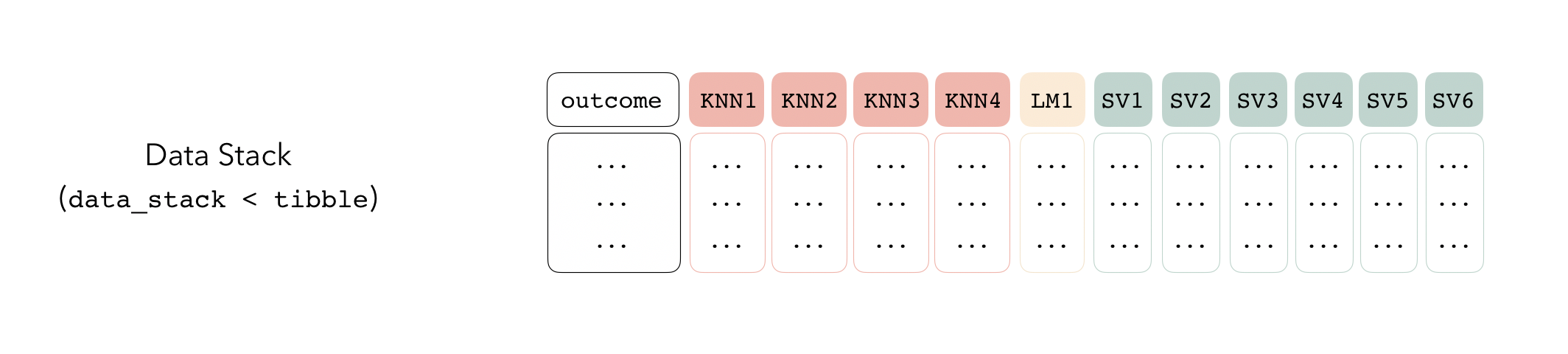
Adding Candidates to a Data Stack
Candidate members first come together in a data_stack object through the add_candidates() function. Principally, these objects are just tibbles, where the first column gives the true outcome in the assessment set, and the remaining columns give the predictions from each candidate ensemble member. (When the outcome is numeric, there’s only one column per candidate ensemble member. Classification requires as many columns per candidate as there are levels in the outcome variable.) They also bring along a few extra attributes to keep track of model definitions.
The first step to building a data stack is the initialization step. The stacks() function works sort of like the ggplot() constructor from ggplot2—the function creates a basic structure that the object will be built on top of—except you’ll pipe the outputs rather than adding them with +.
stacks()## # A data stack with 0 model definitions and 0 candidate members.The add_candidates() function adds candidate ensemble members to the data stack!
wind_data_st <-
  stacks() %>%
  add_candidates(lin_reg_res) %>%
  add_candidates(spline_res) %>%
  add_candidates(svm_res)

wind_data_st
## # A data stack with 3 model definitions and 15 candidate members:
## # lin_reg_res: 1 sub-model
## # spline_res: 9 sub-models
## # svm_res: 5 sub-models
## # Outcome: turbine_rated_capacity_kw (numeric)As mentioned before, under the hood, a data_stack object is really just a tibble with some extra attributes. Checking out the actual data:
as_tibble(wind_data_st)## # A tibble: 4,373 x 16
## turbine_rated_c… lin_reg_res_1_1 spline_res_5_1 spline_res_7_1 spline_res_8_1
## <dbl> <dbl> <dbl> <dbl> <dbl>
## 1 150 -74.5 -116. -434. -437.
## 2 600 502. 483. 407. 465.
## 3 600 662. 638. 555. 573.
## 4 600 649. 631. 537. 556.
## 5 600 690. 665. 580. 579.
## 6 660 731. 709. 656. 664.
## 7 1300 905. 903. 954. 1007.
## 8 1300 956. 949. 985. 1034.
## 9 1300 912. 907. 957. 996.
## 10 1300 940. 936. 988. 1036.
## # … with 4,363 more rows, and 11 more variables: spline_res_2_1 <dbl>,
## # spline_res_3_1 <dbl>, spline_res_4_1 <dbl>, spline_res_1_1 <dbl>,
## # spline_res_6_1 <dbl>, spline_res_9_1 <dbl>, svm_res_1_4 <dbl>,
## # svm_res_1_2 <dbl>, svm_res_1_3 <dbl>, svm_res_1_5 <dbl>, svm_res_1_1 <dbl>That’s it! We’re now ready to evaluate how it is that we need to combine predictions from each candidate ensemble member.
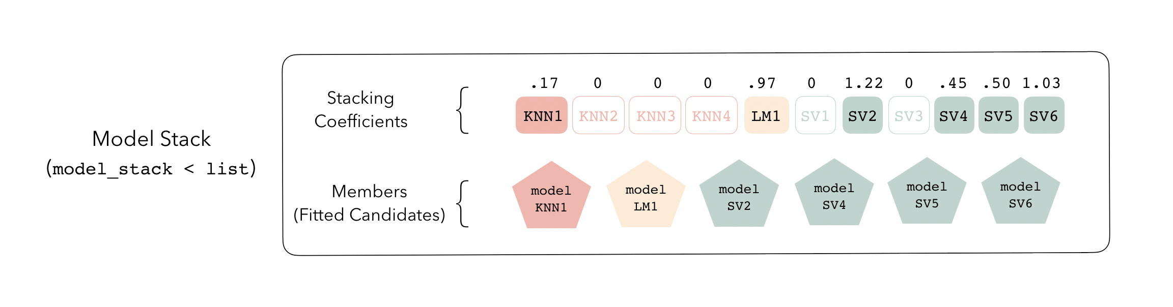
Creating A Model Stack
Then, the data stack can be evaluated using blend_predictions() to determine to how best to combine the outputs from each of the candidate members.
The outputs of each member are likely highly correlated. Thus, depending on the degree of regularization you choose, the coefficients for the inputs of (possibly) many of the members will zero out—their predictions will have no influence on the final output, and those terms will thus be thrown out.

wind_model_st <-
  wind_data_st %>%
  blend_predictions()

wind_model_st
## # A tibble: 3 x 3
## member type weight
## <chr> <chr> <dbl>
## 1 spline_res_9_1 linear_reg 0.737
## 2 svm_res_1_3 svm_rbf 0.323
## 3 svm_res_1_4 svm_rbf 0.000920The blend_predictions function determines how member model output will ultimately be combined in the final prediction, and is how we’ll calculate our stacking coefficients. Now that we know how to combine our model output, we can fit the models that we now know we need on the full training set. Any candidate ensemble member that has a stacking coefficient of zero doesn’t need to be refitted!
wind_model_st <-
  wind_model_st %>%
  fit_members()

wind_model_st
## # A tibble: 3 x 3
## member type weight
## <chr> <chr> <dbl>
## 1 spline_res_9_1 linear_reg 0.737
## 2 svm_res_1_3 svm_rbf 0.323
## 3 svm_res_1_4 svm_rbf 0.000920Now that we’ve fitted the needed ensemble members, our model stack is ready to go! For the most part, a model stack is just a list that contains a bunch of ensemble members and instructions on how to combine their predictions.
This model_stack object is now ready to predict with new data!
Evaluating Performance
Let’s check out how well the model stack performs! Predicting on new data:
wind_test <-
  wind_test %>%
  bind_cols(predict(wind_model_st, .))
Juxtaposing the predictions with the true data:
wind_test %>%
  ggplot() +
  aes(
    x = turbine_rated_capacity_kw,
    y = .pred
  ) +
  geom_point() +
  coord_obs_pred()
Looks like our predictions were pretty strong! How do the stacks predictions perform, though, as compared to the members’ predictions? We can use the type = "members" argument to generate predictions from each of the ensemble members.
member_preds <-
  wind_test %>%
  select(turbine_rated_capacity_kw) %>%
  bind_cols(
    predict(
      wind_model_st,
      wind_test,
      members = TRUE
    )
  )
Now, evaluating the root mean squared error from each model:
colnames(member_preds) %>%
  map_dfr(
    .f = rmse,
    truth = turbine_rated_capacity_kw,
    data = member_preds
  ) %>%
  mutate(member = colnames(member_preds))
## # A tibble: 5 x 4
## .metric .estimator .estimate member
## <chr> <chr> <dbl> <chr>
## 1 rmse standard 0 turbine_rated_capacity_kw
## 2 rmse standard 254. .pred
## 3 rmse standard 260. spline_res_9_1
## 4 rmse standard 642. svm_res_1_4
## 5 rmse standard 337. svm_res_1_3As we can see, the stacked ensemble outperforms each of the member models, though is closely followed by one of the spline members.
Voila! You’ve now made use of the stacks package to predict wind turbine capacity using a stacked ensemble model!
That’s A Wrap!
I appreciate yall checking out this tutorial, and hope you’re stoked to give stacks a try!
If it’s helpful, this is a completed version of the diagram we were putting together throughout this tutorial!

Session Info
sessionInfo()## R version 3.6.3 (2020-02-29)
## Platform: x86_64-apple-darwin15.6.0 (64-bit)
## Running under: macOS Catalina 10.15.4
##
## Matrix products: default
## BLAS: /Library/Frameworks/R.framework/Versions/3.6/Resources/lib/libRblas.0.dylib
## LAPACK: /Library/Frameworks/R.framework/Versions/3.6/Resources/lib/libRlapack.dylib
##
## locale:
## [1] en_US.UTF-8/en_US.UTF-8/en_US.UTF-8/C/en_US.UTF-8/en_US.UTF-8
##
## attached base packages:
## [1] stats graphics grDevices utils datasets methods base
##
## other attached packages:
## [1] glmnet_4.0-2 Matrix_1.2-18 kernlab_0.9-29
## [4] vctrs_0.3.4 rlang_0.4.8 stacks_0.0.0.9000
## [7] yardstick_0.0.7 workflows_0.2.1.9000 tune_0.1.1.9001
## [10] rsample_0.0.8.9000 recipes_0.1.13.9000 parsnip_0.1.3.9000
## [13] modeldata_0.1.0 infer_0.5.3.9000 dials_0.0.9.9000
## [16] scales_1.1.1 broom_0.7.2 tidymodels_0.1.1
## [19] forcats_0.5.0 stringr_1.4.0 dplyr_1.0.2
## [22] purrr_0.3.4 readr_1.4.0 tidyr_1.1.2
## [25] tibble_3.0.4.9000 ggplot2_3.3.2 tidyverse_1.3.0
##
## loaded via a namespace (and not attached):
## [1] colorspace_1.4-1 ellipsis_0.3.1 class_7.3-15 fs_1.5.0
## [5] rstudioapi_0.11 listenv_0.8.0 furrr_0.2.1 farver_2.0.3
## [9] prodlim_2019.11.13 fansi_0.4.1 lubridate_1.7.9 xml2_1.3.2
## [13] codetools_0.2-16 splines_3.6.3 knitr_1.30 jsonlite_1.7.1
## [17] pROC_1.16.2 dbplyr_1.4.4 compiler_3.6.3 httr_1.4.2
## [21] backports_1.1.10 assertthat_0.2.1 cli_2.1.0 htmltools_0.5.0
## [25] tools_3.6.3 gtable_0.3.0 glue_1.4.2 Rcpp_1.0.5
## [29] cellranger_1.1.0 DiceDesign_1.8-1 blogdown_0.21 iterators_1.0.13
## [33] timeDate_3043.102 gower_0.2.2 xfun_0.18 globals_0.13.1
## [37] rvest_0.3.6 lifecycle_0.2.0 future_1.19.1 MASS_7.3-53
## [41] ipred_0.9-9 hms_0.5.3 parallel_3.6.3 yaml_2.2.1
## [45] curl_4.3 rpart_4.1-15 stringi_1.5.3 foreach_1.5.1
## [49] butcher_0.1.2 lhs_1.1.1 hardhat_0.1.4.9000 lava_1.6.8
## [53] shape_1.4.5 pkgconfig_2.0.3 evaluate_0.14 lattice_0.20-38
## [57] labeling_0.4.2 tidyselect_1.1.0 plyr_1.8.6 magrittr_1.5
## [61] bookdown_0.14 R6_2.4.1 generics_0.0.2 DBI_1.1.0
## [65] pillar_1.4.6 haven_2.3.1 withr_2.3.0 survival_3.1-8
## [69] nnet_7.3-12 modelr_0.1.5 crayon_1.3.4.9000 utf8_1.1.4
## [73] rmarkdown_2.5 usethis_1.6.3 grid_3.6.3 readxl_1.3.1
## [77] blob_1.2.1 reprex_0.3.0.9001 digest_0.6.27 GPfit_1.0-8
## [81] munsell_0.5.0